LaTeX example
Example of a co-authored LaTeX paper: source and output
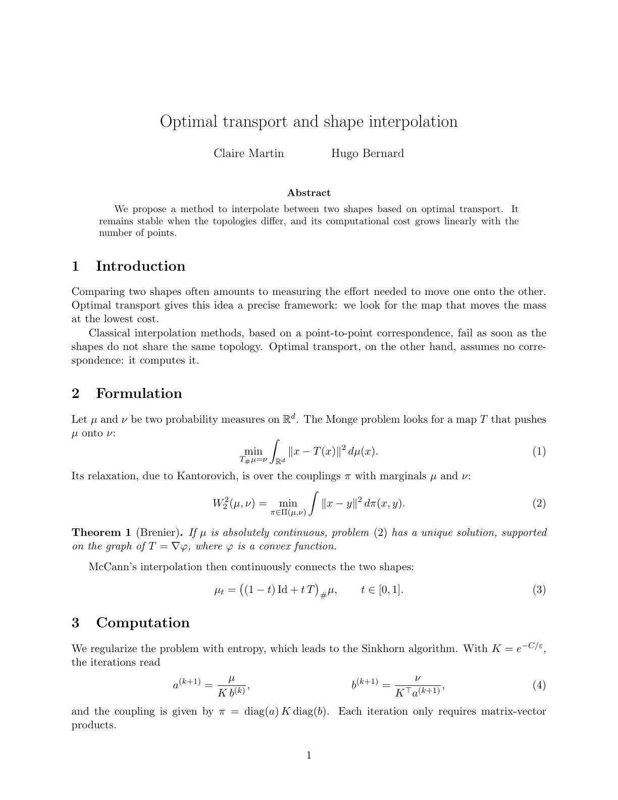
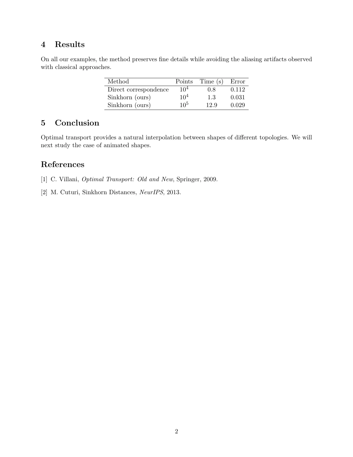
This short paper is sharedraft's demo project. Here is its full LaTeX source, the compiled output, and the review its two co-authors left on it. In the demo, everything can be edited, together and in real time.
What the example contains
“Optimal transport and shape interpolation”: Claire Martin, Hugo Bernard.
articleclass,amsmathandamsthm- Numbered equations,
align, references with\eqref - A theorem (
\newtheorem), atabulartable - Bibliography with
thebibliography
The output
The source
The project's main.tex file, as it opens in the demo.
\documentclass[11pt]{article}
\usepackage[english]{babel}
\usepackage{amsmath,amssymb,amsthm}
\usepackage[margin=2.5cm]{geometry}
\newtheorem{theorem}{Theorem}

\title{Optimal transport and shape interpolation}
\author{Claire Martin \and Hugo Bernard}
\date{}

\begin{document}
\maketitle

\begin{abstract}
We propose a method to interpolate between two shapes based on optimal
transport. It remains stable when the topologies differ, and its computational
cost grows linearly with the number of points.
\end{abstract}

\section{Introduction}
Comparing two shapes often amounts to measuring the effort needed to move one
onto the other. Optimal transport gives this idea a precise framework: we look
for the map that moves the mass at the lowest cost.

Classical interpolation methods, based on a point-to-point correspondence, fail
as soon as the shapes do not share the same topology. Optimal transport, on
the other hand, assumes no correspondence: it computes it.

\section{Formulation}
Let $\mu$ and $\nu$ be two probability measures on $\mathbb{R}^d$. The Monge
problem looks for a map $T$ that pushes $\mu$ onto $\nu$:
\begin{equation}
  \min_{T_\# \mu = \nu} \int_{\mathbb{R}^d} \|x - T(x)\|^2 \, d\mu(x).
\end{equation}
Its relaxation, due to Kantorovich, is over the couplings $\pi$ with marginals
$\mu$ and $\nu$:
\begin{equation}
  W_2^2(\mu,\nu) = \min_{\pi \in \Pi(\mu,\nu)} \int \|x-y\|^2 \, d\pi(x,y).
  \label{eq:kantorovich}
\end{equation}

\begin{theorem}[Brenier]
If $\mu$ is absolutely continuous, problem~\eqref{eq:kantorovich} has a unique
solution, supported on the graph of $T = \nabla \varphi$, where $\varphi$ is a
convex function.
\end{theorem}

McCann's interpolation then continuously connects the two shapes:
\begin{equation}
  \mu_t = \big((1-t)\,\mathrm{Id} + t\,T\big)_\# \mu, \qquad t \in [0,1].
\end{equation}

\section{Computation}
We regularize the problem with entropy, which leads to the Sinkhorn algorithm.
With $K = e^{-C/\varepsilon}$, the iterations read
\begin{align}
  a^{(k+1)} &= \frac{\mu}{K\, b^{(k)}}, &
  b^{(k+1)} &= \frac{\nu}{K^\top a^{(k+1)}},
\end{align}
and the coupling is given by $\pi = \operatorname{diag}(a)\, K \operatorname{diag}(b)$.
Each iteration only requires matrix-vector products.

\section{Results}
On all our examples, the method preserves fine details while avoiding the
aliasing artifacts observed with classical approaches.

\begin{center}
\begin{tabular}{lccc}
  \hline
  Method & Points & Time (s) & Error \\
  \hline
  Direct correspondence & $10^4$ & 0.8 & 0.112 \\
  Sinkhorn (ours) & $10^4$ & 1.3 & 0.031 \\
  Sinkhorn (ours) & $10^5$ & 12.9 & 0.029 \\
  \hline
\end{tabular}
\end{center}

\section{Conclusion}
Optimal transport provides a natural interpolation between shapes of different
topologies. We will next study the case of animated shapes.

\begin{thebibliography}{9}
\bibitem{villani} C.~Villani, \emph{Optimal Transport: Old and New}, Springer, 2009.
\bibitem{cuturi} M.~Cuturi, Sinkhorn Distances, \emph{NeurIPS}, 2013.
\end{thebibliography}
\end{document}
The review in the demo
When you open the demo, the paper has already been reviewed by its two fictional co-authors, Claire and Hugo: threaded comments on the source, marks drawn on the output, and two tracked changes to accept or reject.
Comments
- on “Optimal transport and shape interpolation”Claire: Welcome! This project is shared with every visitor and reset every 20 minutes. Write, comment, annotate the preview: the others see it right away.
- on “at the lowest cost”Claire: Cite Villani here?Hugo: Yes, the 2009 book.
- on “absolutely continuous”Hugo: Key assumption: recall it in the introduction?
- on “Sinkhorn”Claire: Give the value of ε used in the experiments.
- on “aliasing artifacts”Hugo: Add a comparison figure
- on “animated shapes”Claire: Maybe too ambitious for this paper.resolvedHugo: Agreed, let's keep it for later.
Marks on the output
- Bracket in the margin, on “Classical”Hugo: A bit long: tighten this paragraph?
- Zigzag in the margin, on “Brenier”Claire: Check the exact statement (assumptions on μ).
- Note in the margin, on “matrix-vector”Claire: Cost: O(n²) per iteration.
Tracked changes
- Hugo suggests adding “and robust” after “It remains stable”
- Claire suggests deleting “natural”
Try it without an account
The demo is shared by every visitor and reset every 20 minutes: write, comment, annotate, and the others see it right away. Don't put anything personal in it.